Statistical Mechanics

2 Probability

Definition

A probability space consists of a sample space $Ω$ , such that for (some of the) events $E \subset Ω$ , we assign a probability $P (E) \in [0, 1]$ so that

$\cdot$ $P (Ω) = 1$ , and
$\cdot$ if $E_{1} \cap E_{2} = \emptyset$ are disjoint events, then $P (E_{1} \cup E_{2}) = P (E_{1}) + P (E_{2})$ .

basically the usual countable additivity

Definition

The objective probability obtained experimentally from the relative frequency of an occurrence in many tests of the random variable

lim_{n \to \infty} \frac{n_{A}}{n}

where $n$ is the number of times a random process is repeated and $n_{A}$ represents the number of times event $A$ occurs in those $n$ repetitions. Clearly the bigger the $n$ the more accurate

Definition

A real random variable is a map $X : Ω \to R$ , which can also be defined by a cumulative distribution function

F (x) = P ({ω \in Ω : X (ω) \leq x}) = P (X \leq x) .

Definition

The expectation value of a function $g (X)$ , denoted $⟨ g (X) ⟩$ , is

⟨ g (X) ⟩ = \int p (x) g (x) d x .

One specific example is the moments of a random variable X, which are

⟨ X^{m} ⟩ = \int p (x) x^{m} d x .

Definition

The characteristic function of a random variable X is

\tilde{p} (k) \equiv ⟨ e^{- i k X} ⟩ = \int p (x) e^{- i k x} d x .

and because this is a fourier transform we may obtain the distribution function $p (x)$ via fourier inversion theorem

p (x) = \int \frac{1}{2 π} \tilde{p} (k) e^{i k x} d k

now doing a taylor expansion on the characteristic function

The Taylor series of $\tilde{ρ} (k)$ about $k = 0$ is:

\tilde{ρ} (k) = \sum_{m = 0}^{\infty} \frac{k^{m}}{m!} {\frac{d^{m} \tilde{ρ} (k)}{d k^{m}} |}_{k = 0} .

We need to compute the derivatives $\frac{d^{m} \tilde{ρ} (k)}{d k^{m}}$ .

Differentiate under the integral (justified for well-behaved $ρ (x)$ ):

\frac{d^{m} \tilde{ρ} (k)}{d k^{m}} = \frac{d^{m}}{d k^{m}} \int_{- \infty}^{\infty} ρ (x) e^{- i k x} d x = \int_{- \infty}^{\infty} ρ (x) \frac{\partial^{m}}{\partial k^{m}} (e^{- i k x}) d x .

The partial derivative is:

\frac{\partial^{m}}{\partial k^{m}} (e^{- i k x}) = (- i x)^{m} e^{- i k x} .

So:

\frac{d^{m} \tilde{ρ} (k)}{d k^{m}} = \int_{- \infty}^{\infty} ρ (x) (- i x)^{m} e^{- i k x} d x .

Evaluate at $k = 0$ :

{\frac{d^{m} \tilde{ρ} (k)}{d k^{m}} |}_{k = 0} = \int_{- \infty}^{\infty} ρ (x) (- i x)^{m} d x = (- i)^{m} \int_{- \infty}^{\infty} ρ (x) x^{m} d x = (- i)^{m} ⟨ X^{m} ⟩,

where $⟨ X^{m} ⟩ = \int_{- \infty}^{\infty} ρ (x) x^{m} d x$ is the $m$ -th moment. So we have

\tilde{ρ} (k) = \sum_{m = 0}^{\infty} \frac{k^{m}}{m!} (- i)^{m} ⟨ X^{m} ⟩ = \sum_{m = 0}^{\infty} \frac{(- i k)^{m}}{m!} ⟨ X^{m} ⟩ .

Definition

the cumulant generating function is the logarithm of the characteristic function.

\ln \tilde{p} (k) = \sum_{n = 1}^{\infty} \frac{(- i k)^{n}}{n!} ⟨ x^{n} ⟩_{c} .

Proposition

We have

⟨ x^{m} ⟩ = {\sum_{{p_{n}}}}^{'} m! \prod_{n} \frac{1}{p_{n}! (n!)^{p_{n}}} ⟨ x^{n} ⟩_{c}^{p_{n}} .

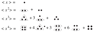
and that we may see the nth cumulant as a connected cluster of n points and the mth moment as the sum of all subdivision of m points into partitions of smaller clusters

first by definition we have

\sum_{m = 0}^{\infty} \frac{(- i k)^{m}}{m!} ⟨ x^{m} ⟩ = \exp [\sum_{n = 1}^{\infty} \frac{(- i k)^{n}}{n!} ⟨ x^{n} ⟩_{c}]

we may rewrite the RHS as

\exp [\sum_{n = 1}^{\infty} \frac{(- i k)^{n}}{n!} ⟨ x^{n} ⟩_{c}] = \prod_{n = 1}^{\infty} \exp (\frac{(- i k)^{n}}{n!} ⟨ x^{n} ⟩_{c})

for each $n$ expand the indivdual exponential using its taylor series

\exp (\frac{(- i k)^{n}}{n!} ⟨ x^{n} ⟩_{c}) = \sum_{p_{n} = 0}^{\infty} \frac{1}{p_{n}!} {(\frac{(- i k)^{n}}{n!} ⟨ x^{n} ⟩_{c})}^{p_{n}}

simplify to get for each $n$

\frac{1}{p_{n}!} {(\frac{(- i k)^{n}}{n!} ⟨ x^{n} ⟩_{c})}^{p_{n}} = \frac{(- i k)^{n p_{n}}}{p_{n}!} {(\frac{⟨ x^{n} ⟩_{c}}{n!})}^{p_{n}} = \frac{(- i k)^{n p_{n}} ⟨ x^{n} ⟩_{c}^{p_{n}}}{p_{n}! (n!)^{p_{n}}}

so altogether we get

\sum_{m = 0}^{\infty} \frac{(- i k)^{m}}{m!} ⟨ x^{m} ⟩ = \prod_{n = 1}^{\infty} [\sum_{p_{n} = 0}^{\infty} \frac{(- i k)^{n p_{n}} ⟨ x^{n} ⟩_{c}^{p_{n}}}{p_{n}! (n!)^{p_{n}}}]

now we equate the coefficients of $(- i k)^{m}$ in which case for each $m$ the contribution by the LHS and RHS respectively is

\frac{⟨ x^{m} ⟩}{m!} = \sum_{{p_{n}} : \sum n p_{n} = m} \prod_{n} \frac{⟨ x^{n} ⟩_{c}^{p_{n}}}{p_{n}! (n!)^{p_{n}}}

rearranging this gives the desired result

now $\sum_{{p_{n} : \sum n p_{n} = m}}$ simply counts the number of ways to break $m$ points into ${p_{n}}$ clusters/partitions of $n$ points where each $p_{n}$ value represents the multiplicity of a partition of size $n$ .

Remark

Above it also serves to select chosen values of $p_{n}$ for each $n$ . Then $\prod_{n}$ simply multiplies these pre-selected set ${p_{n}}$
next notice that for each chosen way of partitioning we divide by $p_{n}!$ and $(n!)^{p_{n}}$ as we don't want to repeat count clusters and the balls in each cluster

Example

graphically
../../../Attachments/Pasted image 20250721054041.png
corresponds to

⟨ x ⟩ = ⟨ x ⟩_{c},

⟨ x^{2} ⟩ = ⟨ x^{2} ⟩_{c} + ⟨ x ⟩_{c}^{2},

⟨ x^{3} ⟩ = ⟨ x^{3} ⟩_{c} + 3 ⟨ x^{2} ⟩_{c} ⟨ x ⟩_{c} + ⟨ x ⟩_{c}^{3},

⟨ x^{4} ⟩ = ⟨ x^{4} ⟩_{c} + 4 ⟨ x^{3} ⟩_{c} ⟨ x ⟩_{c} + 3 ⟨ x^{2} ⟩_{c}^{2} + 6 ⟨ x^{2} ⟩_{c} ⟨ x ⟩_{c}^{2} + ⟨ x ⟩_{c}^{4} .

2.3 Some Important Probability Distributions

Definition

the normal(gaussian) distribution describes a continuous real random variable $x$ with

p (x) = \frac{1}{\sqrt{2 π σ^{2}}} \exp [- \frac{(x - λ)^{2}}{2 σ^{2}}] .

Proposition

the corresponding characteristic function is then

\tilde{p} (k) = \int_{- \infty}^{\infty} d x \frac{1}{\sqrt{2 π σ^{2}}} \exp [- \frac{(x - λ)^{2}}{2 σ^{2}} - i k x] = \exp [- i k λ - \frac{k^{2} σ^{2}}{2}] .

proof: essentially group all $x$ terms into a quadratic form so that we may apply the standard gaussian integral result. Specifically we first expand the exponent

- \frac{x^{2}}{2 σ^{2}} + \frac{λ x}{σ^{2}} - \frac{λ^{2}}{2 σ^{2}} - i k x = - \frac{x^{2}}{2 σ^{2}} + (\frac{λ}{σ^{2}} - i k) x - \frac{λ^{2}}{2 σ^{2}}

then letting the terms in the paranthesis be $b$ we rearrange to get

- \frac{1}{2 σ^{2}} (x^{2} - 2 σ^{2} b x) - \frac{λ^{2}}{2 σ^{2}}

basically with the goal of separating the $x$ from the constants in the exponent. Then finally to get the gaussian integral form we need a quadratic factorization of $x$ so we do complete the square in the paranthesis to get

- \frac{1}{2 σ^{2}} [(x - σ^{2} b)^{2} - (σ^{2} b)^{2}] - \frac{λ^{2}}{2 σ^{2}} = - \frac{(x - σ^{2} b)^{2}}{2 σ^{2}} + \frac{σ^{2} b^{2}}{2} - \frac{λ^{2}}{2 σ^{2}} .

we sub back $b$ into the constant part

\frac{σ^{2} b^{2}}{2} - \frac{λ^{2}}{2 σ^{2}} = \frac{λ^{2}}{2 σ^{2}} - i k λ - \frac{k^{2} σ^{2}}{2} - \frac{λ^{2}}{2 σ^{2}} = - i k λ - \frac{k^{2} σ^{2}}{2} .

and then separate out $x$ and the constants in the exponent as desired

\tilde{ρ} (k) = \frac{1}{\sqrt{2 π σ^{2}}} \exp (- i k λ - \frac{k^{2} σ^{2}}{2}) \int_{- \infty}^{\infty} \exp [- \frac{(x - σ^{2} b)^{2}}{2 σ^{2}}] d x .

as planned we recognize the gaussian integral form in the integral on the right and therefore we have

\tilde{ρ} (k) = \frac{1}{\sqrt{2 π σ^{2}}} \exp (- i k λ - \frac{k^{2} σ^{2}}{2}) \cdot \sqrt{2 π σ^{2}} = \exp (- i k λ - \frac{k^{2} σ^{2}}{2})

and so cumulants are in the form

\ln \tilde{p} (k) = - i k λ - k^{2} σ^{2} / 2,

so it is clear by comparing with the definition above that

⟨ x ⟩_{c} = λ, ⟨ x^{2} ⟩_{c} = σ^{2}, ⟨ x^{3} ⟩_{c} = ⟨ x^{4} ⟩_{c} = \dots = 0

in which case calcuation of moments from the culmulants using the previous proposition is just

⟨ x ⟩ = λ,

⟨ x^{2} ⟩ = σ^{2} + λ^{2},

⟨ x^{3} ⟩ = 3 σ^{2} λ + λ^{3},

⟨ x^{4} ⟩ = 3 σ^{4} + 6 σ^{2} λ^{2} + λ^{4},

Definition

the binomial distribution consider a random variable with two outcomes $A$ and $B$ of relative probabilities $p_{A}$ and $p_{B} = 1 - p_{A}$ then the probability $A$ occurs $N_{A}$ times in $N$ trials is

p_{N} (N_{A}) = (\binom{N}{N_{A}}) p_{A}^{N_{A}} p_{B}^{N - N_{A}}

note that we have

(\binom{N}{N_{A}}) = \frac{N!}{N_{A}! (N - N_{A})!}

then our characteristic function is given by(the 3rd equality follows because the LHS is simply the binomial expansion of the RHS)

{\tilde{p}}_{N} (k) = ⟨ e^{- i k N_{A}} ⟩ = \sum_{N_{A} = 0}^{N} \frac{N!}{N_{A}! (N - N_{A})!} p_{A}^{N_{A}} p_{B}^{N - N_{A}} e^{- i k N_{A}} = {(p_{A} e^{- i k} + p_{B})}^{N} .

and consequently our cumulent generating function is

\ln {\tilde{p}}_{N} (k) = N \ln (p_{A} e^{- i k} + p_{B}) = N \ln {\tilde{p}}_{1} (k),

Definition

the poisson distribution

2.4 Many Random Variables

Definition

the **joint PDF ** $p (x)$ is the probability density of an outcome in a volume element $d^{N} x = \prod_{i = 1}^{N} d x_{i}$ around the point $x = {x_{1}, x_{2}, \dots, x_{N}}$

in other words, letting $X$ be a vector of random variables:

p (\vec{x}) = lim_{\forall i, d x_{i} \to 0} \frac{P (\vec{X} is in the box around \vec{x} of width \prod_{i} d x_{i})}{d x_{1} d x_{2} \dots d x_{N}} .

the joint PDF is normalized such that

p_{x} (S) = \int d^{N} x p (x) = 1

if and only if the $N$ random variables are independent the joint PDF is then the product of individual PDFs

p (x) = \prod_{i = 1}^{N} p_{i} (x_{i})

Definition

the unconditional PDF describes the subset of random variables independent of the values of others. For example you are only interested in the first $m$ variables of the $N$ total variables then:

p (x_{1}, . . ., x_{m}) = \int \prod_{i = m + 1}^{N} d x_{i} p (x_{1}, . . ., x_{N}) .

where effectively we have integrated over all the other non-relevant variables for each ${x_{1}, \dots, x_{m}}$ .

Observe that now our PDF does not depend on the variables ${x_{m + 1}, \dots, x_{N}}$ as they are automatically included for any ${x_{1}, \dots, x_{m}}$ . For example say we have position vector $(x, y, z)$ and we are only interested in $(x)$ . The unconditional PDF simply includes all probability density contributions over $(y, z)$ for each $x$ so our PDF is independent of $y, z$

Definition

the conditional PDF describes the behavior of a subset of random variables for specified values of others. For example consider $p (\vec{x}, \vec{v}) / N = p (\vec{v} | \vec{x})$ where $p (\vec{x}, \vec{v})$ is the joint PDF and that $p (\vec{v} | \vec{x})$ is the conditional PDF for velocity $\vec{v}$ at a given fixed position $\vec{x}$

note we have $N$ , a normalization factor that ensures

\int p (\vec{x}, \vec{v}) / N d^{3} v = \int p (\vec{v} | \vec{x}) d^{3} v = 1

so we have

N = \int d^{3} \vec{v} p (\vec{x}, \vec{v}) = p (\vec{x}),

where the final equality follows because the 2nd expression is simply the definition of unconditional PDF as defined just previously!

Proposition

Essentially we have just shown that Bayes' Theorem

p (x_{1}, \dots, x_{m} | x_{m + 1}, \dots, x_{N}) = \frac{p (x_{1}, \dots, x_{N})}{p (x_{m + 1}, \dots, x_{N})} .

Definition

the expectation value of a function $F (x)$ is obtained as before from

⟨ F (x) ⟩ = \int d^{N} x p (x) F (x) .

and the joint characteristic function will then be the N-dimensional Fourier Transformationn of the joint PDF

\tilde{p} (k) = ⟨ \exp (- i \sum_{j = 1}^{N} k_{j} x_{j}) ⟩ .

= \int_{- \infty}^{\infty} \dots \int_{- \infty}^{\infty} p (x_{1}, \dots, x_{N}) \exp (- i \sum_{j = 1}^{N} k_{j} x_{j}) d x_{1} \dots d x_{N} .

like before we do a taylor expression but this time for a multivariate case

\exp (- i \sum_{j = 1}^{N} k_{j} x_{j}) = \sum_{m = 0}^{\infty} \frac{1}{m!} {(- i \sum_{j = 1}^{N} k_{j} x_{j})}^{m}

we may now apply the multinomial expansion given by

{(\sum_{j = 1}^{N} k_{j} x_{j})}^{m} = \sum_{n_{1} + \dots + n_{N} = m} \frac{m!}{n_{1}! \dots n_{N}!} (k_{1} x_{1})^{n_{1}} \dots (k_{N} x_{N})^{n_{N}},

where we may sub into our expression to get

\exp (- i \sum_{j = 1}^{N} k_{j} x_{j}) = \sum_{m = 0}^{\infty} \frac{(- i)^{m}}{m!} \sum_{n_{1} + \dots + n_{N} = m} \frac{m!}{n_{1}! \dots n_{N}!} (k_{1} x_{1})^{n_{1}} \dots (k_{N} x_{N})^{n_{N}} .

= \sum_{m = 0}^{\infty} \sum_{n_{1} + \dots + n_{N} = m} \frac{(- i)^{m}}{n_{1}! \dots n_{N}!} (k_{1} x_{1})^{n_{1}} \dots (k_{N} x_{N})^{n_{N}} .

with this we may rewrite our characteristic function $\tilde{p} (k)$ like so

\tilde{p} (k) = E [\sum_{m = 0}^{\infty} \sum_{n_{1} + \dots + n_{N} = m} \frac{(- i)^{m}}{n_{1}! \dots n_{N}!} (k_{1} x_{1})^{n_{1}} \dots (k_{N} x_{N})^{n_{N}}]

= \sum_{m = 0}^{\infty} \sum_{n_{1} + \dots + n_{N} = m} \frac{(- i)^{m}}{n_{1}! \dots n_{N}!} k_{1}^{n_{1}} \dots k_{N}^{n_{N}} E [x_{1}^{n_{1}} \dots x_{N}^{n_{N}}] .

where $E [x_{1}^{n_{1}} \dots x_{N}^{n_{N}}] = ⟨ x_{1}^{n_{1}} \dots x_{N}^{n_{N}} ⟩$ (inside is a product btw). With these the following should make sense

Example

consider

\frac{\partial}{\partial (- i k_{1})} \tilde{p} (k) |_{k = 0} = \int_{- \infty}^{\infty} \dots \int_{- \infty}^{\infty} p (x_{1}, \dots, x_{N}) \exp (- i \sum_{j = 1}^{N} k_{j} x_{j}) x_{1} d x_{1} \dots d x_{N} = ⟨ x_{1} ⟩ |_{k = 0}

= \int_{- \infty}^{\infty} \dots \int_{- \infty}^{\infty} x_{1} p (x_{1}, \dots, x_{N}) \cdot 1 d x_{1} \dots d x_{N} = ⟨ x_{1} ⟩,

Example

and consider in general

⟨ x_{1}^{n_{1}} x_{2}^{n_{2}} \dots x_{N}^{n_{N}} ⟩ = {[\frac{\partial}{\partial (- i k_{1})}]}^{n_{1}} {[\frac{\partial}{\partial (- i k_{2})}]}^{n_{2}} \dots {[\frac{\partial}{\partial (- i k_{N})}]}^{n_{N}} \tilde{p} (k = 0),

similarly for cumlants we have

⟨ X_{1}^{m_{1}} X_{2}^{m_{2}} \dots X_{n}^{m_{n}} ⟩_{c} = {(\frac{\partial}{\partial (- i k_{1})})}^{m_{1}} \dots {(\frac{\partial}{\partial (- i k_{n})})}^{m_{n}} (\ln \tilde{ρ} (\vec{k})) |_{\vec{k} = 0} .

which should make sense if you recall how cumulants are defined.

Example

The same "points in bags" argument for relating cumulants and moments works here: if we want to put two 1s and one 2 into bags, the different configurations are (112), two ways for (1)(12), one way for (2)(11), and one way for (1)(1)(2), so

⟨ X_{1}^{2} X_{2} ⟩ = ⟨ X_{1}^{2} X_{2} ⟩_{c} + 2 ⟨ X_{1} ⟩_{c} ⟨ X_{1} X_{2} ⟩_{c} + ⟨ X_{2} ⟩_{c} ⟨ X_{1}^{2} ⟩_{c} + ⟨ X_{1} ⟩_{c}^{2} ⟨ X_{2} ⟩_{c} .

Proposition

The joint gaussian distribution in N dimensions is given by

p (x) = \frac{1}{\sqrt{(2 π)^{N} det [C]}} \exp [- \frac{1}{2} \sum_{m n} {(C^{- 1})}_{m n} (x_{m} - λ_{m}) (x_{n} - λ_{n})]

Proof: first recall the univariate gaussian distribution but this time suppose we have N independent univariate guassian random variables $x_{1}, x_{2}, \dots, x_{N}$ each with its own mean $λ_{j}$ and variance $σ_{j}^{2}$ . The PDF for each $x_{j}$ is then:

p_{j} (x_{j}) = \frac{1}{\sqrt{2 π σ_{j}^{2}}} \exp [- \frac{(x_{j} - λ_{j})^{2}}{2 σ_{j}^{2}}]

since they are independent we have for $x = (x_{1}, \dots, x_{N})^{T}$

p (x) = \prod_{j = 1}^{N} p_{j} (x_{j}) = \prod_{j = 1}^{N} \frac{1}{\sqrt{2 π σ_{j}^{2}}} \exp [- \frac{(x_{j} - λ_{j})^{2}}{2 σ_{j}^{2}}]

which we may simplify to

p (x) = \frac{1}{(2 π)^{N / 2} \sqrt{\prod_{j = 1}^{N} σ_{j}^{2}}} \exp [- \frac{1}{2} \sum_{j = 1}^{N} \frac{(x_{j} - λ_{j})^{2}}{σ_{j}^{2}}]

in matrix form we may write

- \frac{1}{2} \sum_{j = 1}^{N} \frac{(x_{j} - λ_{j})^{2}}{σ_{j}^{2}} = - \frac{1}{2} (x - λ)^{T} C^{- 1} (x - λ),

where $C = diag (σ_{1}^{2}, σ_{2}^{2}, \dots, σ_{N}^{2})$ and $λ = (λ_{1}, \dots, λ_{N})^{T}$ . Therefore we may also rewrite this as

p (x) = \frac{1}{\sqrt{(2 π)^{N} det [C]}} \exp [- \frac{1}{2} (x - λ)^{T} C^{- 1} (x - λ)]

as for the characteristic function first recall that

\tilde{p} (k) = \int_{- \infty}^{\infty} \dots \int_{- \infty}^{\infty} p (x) \exp (- i \sum_{j = 1}^{N} k_{j} x_{j}) d x_{1} \dots d x_{N}

so substituting the join PDF we obtain

\tilde{p} (k) = \int [\prod_{j = 1}^{N} p_{j} (x_{j})] \exp (- i \sum_{j = 1}^{N} k_{j} x_{j}) d x = \prod_{j = 1}^{N} [\int p_{j} (x_{j}) e^{- i k_{j} x_{j}} d x_{j}] = \prod_{j = 1}^{N} {\tilde{p}}_{j} (k_{j})

now for each ${\tilde{p}}_{j} (k_{j})$ recall from earlier we should then get

\tilde{p} (k) = \prod_{j = 1}^{N} \exp [- i k_{j} λ_{j} - \frac{1}{2} σ_{j}^{2} k_{j}^{2}] = \exp [- i \sum_{j = 1}^{N} k_{j} λ_{j} - \frac{1}{2} \sum_{j = 1}^{N} σ_{j}^{2} k_{j}^{2}]

finally to get the matrix form we first define the mean vector $λ = (λ_{1}, . . ., λ_{N})^{T}$ and wavevector $k = (k_{1}, . . ., k_{N})^{T}$ . The linear term is

\sum_{j = 1}^{N} k_{j} λ_{j} = k^{T} λ .

For the quadratic term, since variables are independent, the covariance matrix $C$ is
diagonal: $C = ⟨ diag (σ_{1}^{2}, . . ., σ_{N}^{2}), so:$

\sum_{j = 1}^{N} σ_{j}^{2} k_{j}^{2} = \sum_{m, n = 1}^{N} C_{m n} k_{m} k_{n} = k^{T} C k,

(with off-diagonals zero). Thus:

\tilde{p} (k) = \exp [- i k^{T} λ - \frac{1}{2} k^{T} C k]

comparing with the univariate case that we will have

⟨ x_{m} ⟩_{c} = λ_{m}, ⟨ x_{m} x_{n} ⟩_{c} = C_{m n},

Theorem

Wick's theorem says that suppose we have a multivariate Guassian with $\vec{λ} = 0$ then

⟨ X_{1}^{m_{1}} \dots X_{n}^{m_{n}} ⟩ = {\begin{cases} 0 & \sum m_{i} is odd \\ sum over all pairwise contractions & otherwise \end{cases}

proof: study quantum field theory first...for now just assume this

We now will like to consider functions of random variables. First consider

\int_{a}^{b} p_{Y} (y) d y = \int_{- \infty}^{\infty} d x p_{X} (x) 1_{[a, b]} (g (x))

where $Y = g (X)$ and $1_{[a, b]}$ is the indicator function that returns if $g (x)$ is in the range $[a, b]$ and 0 otherwise. We can rewrite this as

= \int_{- \infty}^{\infty} d x p_{X} (x) \int_{a}^{b} δ (g (x) - y) d y

now because $a, b$ is arbitrary then have

p_{Y} (y) = \int_{- \infty}^{\infty} d x p_{X} (x) δ (g (x) - y) .

with this relation we may easily generalize to multi-dimensions like so

ρ_{Y} (y) = \int (\prod_{i} d x_{i}) ρ (x_{1}, \dots, x_{n}) δ (g (x_{1}, \dots, x_{n}) - y) .

Example

Let $Y = X_{1}^{2} + X_{2}^{2}$ , where $X_{1}, X_{2}$ are independent random variables.

Then we can write the probability distribution function as

p_{Y} (y) = \int d x_{1} d x_{2} p_{1} (x_{1}) p_{2} (x_{2}) δ (x_{1}^{2} + x_{2}^{2} - y),

and this can be simplified most easily by using a (polar) change of variables: set

r^{2} = x_{1}^{2} + x_{2}^{2} ⟹ d x_{1} d x_{2} = r d r d θ = \frac{1}{2} d θ d (r^{2}),

so that $x_{1} = r \cos θ$ and $x_{2} = r \sin θ$ . Then

p_{Y} (y) = \int \frac{1}{2} d θ d (r^{2}) p_{1} (r \cos θ) p_{2} (r \sin θ) δ (r^{2} - y),

and now we can plug in $r^{2} = y ⟹ r = \sqrt{y}$ (in polar coordinates, r is always nonnegative) wherever it appears to get

p_{Y} (y) = \int_{0}^{2 π} \frac{d θ}{2} p_{1} (\sqrt{y} \cos θ) p_{2} (\sqrt{y} \sin θ),

and we've removed the delta function from the expression.

3 Kinetic Theory of gases

Kinetic theory studies the macroscopic properties of large numbers of particles, starting from their (classical) equations of motion.

First we consider how to define "equilibrium" for a system of particles. Consider a dilute(nearly ideal) gas.

At any time $t$ , the microstate of a system of N particles is described by specifying the positions ${\vec{q}}_{i} (t)$ and momenta ${\vec{p}}_{i} (t)$ of all particles.

The micostate corresponds to a point $μ (t)$ in the 6-N dimensional phase space $Γ = \prod_{i = 1}^{N} {{\vec{q}}_{i}, {\vec{p}}_{i}}$

Fact

Thee time evolution of this point is governed by the canonical equations

${\begin{cases} \frac{d {\vec{q}}_{i}}{d t} = \frac{\partial H}{\partial {\vec{p}}_{i}} \\ \frac{d {\vec{p}}_{i}}{d t} = - \frac{\partial H}{\partial {\vec{q}}_{i}} \end{cases}$

where the hamiltonian $H (p, q)$ describes the total energy in terms of the set of coordinates $q \equiv {{\vec{q}}_{1}, {\vec{q}}_{2}, \dots, {\vec{q}}_{N}}$ and momenta $p \equiv {{\vec{p}}_{1}, {\vec{p}}_{2}, \dots, {\vec{p}}_{N}}$

Now as formulated within thermodynamics the macrostate M of an ideal gas in equilibrium is described by a small number of state functions such as $E, T, P, N$ .

Fact

Many different microstates can represent the same macrostate(i.e a many to one relationship).This is because particles can be arranged in countless ways (positions and velocities) while still giving the same average properties like temperature or pressure

Consider $N$ copies of a particular macrostate each described by a different representative point $μ (t)$ in the phase space $Γ$ .

Definition

A phase space density $ρ (p, q, t)$ is defined by

ρ (p, q, t) d Γ = lim_{N \to \infty} \frac{d N (p, q, t)}{N}

to make sense of this essentially there are $N$ microstates in the phase space $Γ$ . There are $d N$ microstates contained the infinitesimal area $d Γ$ around the point $(p, q)$ . Therefore $lim_{N \to \infty} \frac{d N}{N}$ represents the objective probability(defined above)

knowing this it is then clear that we must have $\int d Γ ρ = 1$ when integrating over the whole phase space $Γ$ for $ρ$ to be a properly normalized probability density function. With these we now define

Definition

Essemble averages for an arbitrary function $O (p, q)$

⟨ O ⟩ = \int d Γ ρ (p, q, t) O (p, q)

Definition

When the exact microstate $μ$ is specified the system is said to be in pure state

On the other hand when our knowledge of the system is probabilistic in a sense that it is take from an density with density $ρ (Γ)$ it is said to be in a mixed state

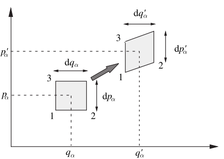
3.2 Liouville's Theorem

Theorem

Liouville's theorem states that the phase space density $ρ (Γ, t)$ behaves like an incompressible fluid

First consider

../../../Attachments/Pasted image 20250717010847.png

In the time interval $δ t$ we have $(p, q) \to (p^{'}, q^{'})$ like so

$q_{α}^{'} = q_{α} + {\dot{q}}_{α} δ t + O (δ t^{2}), p_{α}^{'} = p_{α} + {\dot{p}}_{α} δ t + O (δ t^{2}) .$

which is essentially a taylor expansion 1st order.

Now consider the case for $q$ first. Let 2 points $A, B$ separated by $d q_{α}$ . Then take their time evolutions after $δ t$ :

For Point A:
$q_{α}^{' (A)} = q_{α} + {\dot{q}}_{α} (q_{α}) δ t + O (δ t^{2}) .$
For Point B:

q_{α}^{' (B)} = (q_{α} + d q_{α}) + {\dot{q}}_{α} (q_{α} + d q_{α}) δ t + O (δ t^{2}) .

Since $d q_{α}$ is small, expand ${\dot{q}}_{α}$ around $q_{α}$ :

{\dot{q}}_{α} (q_{α} + d q_{α}) = {\dot{q}}_{α} (q_{α}) + \frac{\partial {\dot{q}}_{α}}{\partial q_{α}} d q_{α} + O (d q_{α}^{2}) .

Plug this into Point B's evolution:

q_{α}^{' (B)} = q_{α} + d q_{α} + [{\dot{q}}_{α} (q_{α}) + \frac{\partial {\dot{q}}_{α}}{\partial q_{α}} d q_{α}] δ t + O (δ t^{2}) .

d q_{α}^{'} = q_{α}^{' (B)} - q_{α}^{' (A)} .

Substitute the expressions:

d q_{α}^{'} = [q_{α} + d q_{α} + {\dot{q}}_{α} (q_{α}) δ t + \frac{\partial {\dot{q}}_{α}}{\partial q_{α}} d q_{α} δ t + O (δ t^{2})] - [q_{α} + {\dot{q}}_{α} (q_{α}) δ t + O (δ t^{2})] .

Simplify and doing everything we have done so far for $q_{α}$ for $p_{α}$ we get

{\begin{cases} d q_{α}^{'} = d q_{α} + \frac{\partial {\dot{q}}_{α}}{\partial q_{α}} d q_{α} δ t + O (δ t^{2}) \\ d p_{α}^{'} = d p_{α} + \frac{\partial {\dot{p}}_{α}}{\partial p_{α}} d p_{α} δ t + O (δ t^{2}) \end{cases} .

we note that $d Γ^{'} = \prod_{i = 1}^{N} d^{3} {\vec{p}}_{i}^{'} d^{3} {\vec{q}}_{i}^{'}$ but we have

d q_{α}^{'} \cdot d p_{α}^{'} = d q_{α} \cdot d p_{α} [1 + (\frac{\partial {\dot{q}}_{α}}{\partial q_{α}} + \frac{\partial {\dot{p}}_{α}}{\partial p_{α}}) δ t + O (δ t^{2})] .

However the time evolution of coordinates and momenta are governed by canonical equations where we have

\frac{\partial {\dot{q}}_{α}}{\partial q_{α}} = \frac{\partial}{\partial q_{α}} \frac{\partial H}{\partial p_{α}} = \frac{\partial^{2} H}{\partial p_{α} \partial q_{α}}, and \frac{\partial {\dot{p}}_{α}}{\partial p_{α}} = \frac{\partial}{\partial p_{α}} (- \frac{\partial H}{\partial q_{α}}) = - \frac{\partial^{2} H}{\partial q_{α} \partial p_{α}} .

therefore

d q_{α}^{'} \cdot d p_{α}^{'} \approx 1

that is $d Γ^{'} = d Γ$ or that in $δ t$ we had $(p, q) \to (p^{'}, q^{'})$ but the volume that $d N$ occupies is the same

Fact

more precisely $ρ$ behaves like the density of an incompressible fluid

The incompressibility condition $ρ (p^{'}, q^{'}, t + δ t) = ρ (p, q, t)$ can be written in differential form as

\frac{d ρ}{d t} = \frac{\partial ρ}{\partial t} + \sum_{α = 1}^{3 N} (\frac{\partial ρ}{\partial p_{α}} \cdot \frac{d ρ_{α}}{d t} + \frac{\partial ρ}{\partial q_{α}} \cdot \frac{d q_{α}}{d t}) = 0.

now subbing above to this equation we obtain

\frac{\partial ρ}{\partial t} = \sum_{α = 1}^{3 N} (\frac{\partial ρ}{\partial p_{α}} \cdot \frac{\partial H}{\partial q_{α}} - \frac{\partial ρ}{\partial q_{α}} \cdot \frac{\partial H}{\partial p_{α}}) = - {ρ, H},

in equilibrium we should have $\frac{\partial}{\partial t} ρ_{eq} = 0$ so from above this means we have ${ρ_{eq}, H} = 0$

Definition

The poisson bracket is defined as

{A, B} \equiv \sum_{α = 1}^{3 N} (\frac{\partial A}{\partial q_{α}} \cdot \frac{\partial B}{\partial p_{α}} - \frac{\partial A}{\partial p_{α}} \cdot \frac{\partial B}{\partial q_{α}}) = - {B, A} .

we used to rewrite our incompressiblity relation as above

Question

so what are the consequences of liouville's theorem ?

4. Classical Statistical Mechanics

2 Probability

2.3 Some Important Probability Distributions

2.4 Many Random Variables

3 Kinetic Theory of gases

3.2 Liouville's Theorem

4. Classical Statistical Mechanics

4.2 The microcanonical ensemble